Clinical examination of the disc has been the basis of disc and nerve fibre layer evaluation for ages but it is marred by its subjectivity and non-reproducibility, in the diagnosis and detection of glaucoma. Though visual field changes give concrete and reproducible evidence of glaucomatous changes, it becomes manifest only after considerable damage has occurred to the retinal ganglion cells(RGCs) and the nerve fibre layer(NFL). There are normally 1.2 - 2.4 million nerve fibres and corresponding number of ganglion cells in the retina. Kerrigan-Baumann and Quigley et al 1 documented that a loss of 35.7% of the RGCs was required for the manifestation of corrected pattern standard deviation(CPSD) <0.5% in the visual fields and a loss of 5dB in the sensitivity was associated with 25% loss in the RGCs. This was because even when some RGCs were dead, surrounding RGCs subserving the same area signal the presence of the target. This stage of glaucoma undetected by conventional Standard white-on-white automated perimetry is known as Pre-perimetric glaucoma.

Thus arose the need to devise methods and technology to detect the presence of pre-perimetric glaucoma and be able to control the disease before it does considerable damage.

The pre-perimetric tools known to us till date are: Frequency Doubling Perimetry (FDP), Heidelberg Retina Tomogram (HRT) and Retinal Nerve Fibre Analysers such as Optical Coherence Tomogram and GDx. We will be discussing each of these by turn.

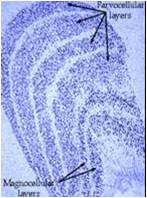
Fig1:Cross-sectional view of lateral geniculate body

Frequency Doubling Perimetry (FDP):

There are two types of RGCs, M type (10% of total RGCs) and P type. The M type cells detect low contrast and high temporal frequency (motion) and project to the Magnocellular layer of Lateral geniculate body. The P cells are responsible for high contrast and low temporal frequency (or static) and project to the Parvocellular layer of Lateral geniculate body.

The larger diameter M cells are the first to die in glaucoma and they form the basis of FDT, which detects this damage whereas standard automated perimetry cannot pick it up.2

A low spatial frequency sinusoidal grating with alternating wide light and dark bars is the stimulus, which undergoes high temporal frequency counter phase flicker i.e. the black bands reverse to become white and the white bands reverse to become black in rapid sequence. The grating, thus, appears to have twice as many light/dark bars i.e. its spatial frequency appears doubled.

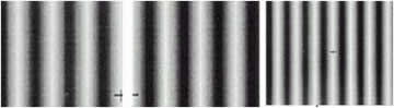
Figure2: Frequency doubling of the target

It is these vulnerable M cells that are thought to transmit signals related to the above target, thereby identifying earlier retinal neuron loss due to glaucoma. FDT is not affected by external room illumination or variations in pupil size. It offers screening (C20) and threshold (N20, N30) programs. On the center of the screen, a black dot is seen for the patient to fixate, and whenever the grating (5 degrees square) is seen in the field (17 locations), the button is pressed.

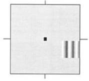
Figure3: The screen of the FDT test

Based upon the contrast required to perceive gratings, a threshold is estimated at the locations tested.
Screening program (C20):

Abnormal screening is considered when either of the following is seen
a) Any defect in the central 5 locations
b) Two mild or moderate defects in the outer 12 locations
c) One severe defect in the outer 12 locations
d) Screening test time > 90 seconds per eye

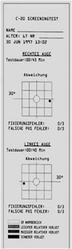
Figure4: Print out of a normal C20 programme

Threshold program (N20 and N30):

This program uses more contrast levels to search for the patient's threshold at each of the tested location. N30- horizontal area extended to include an extra portion of the nasal visual field, resulting in a total 30 degree horizontal field.

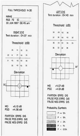
Figure5: Print out of a N30 program

Heidelberg Retinal Tomogram (HRT):

It is based on the principle of confocal scanning laser system which provides 3-D images of the optic nerve head at different planes that are then analysed to give various valuable parameters describing different aspects of the disc. Laser is used as the light source, that when reflected back from the retina is split and detected by two separate detectors to give a 2-D image.

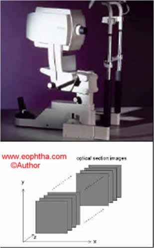
Figure6: The HRT machine (above) and the progressive sections it takes at different levels (below).

When the focal plane is progressively moved deeper to the surface of the retina, 2-D images at different depths produce a 3-D image.

The first focal plane is in the vitreous which is represented as dark. As the focal plane moves posteriorly, it becomes brighter, being the brightest on the retinal surface. The more posterior the plane goes, retina becomes darker and the base of the optic disc cup becomes bright.

Figure7: False color coding of the sections at various levels of depth

The excursion of the focal planes occurs over a range of 2.5millimeters. A total series of 32 images are scanned in a short time span of 1.6 seconds. HRT images have false colour coding, prominent structures are dark and depressed structures are brighter. A manually drawn contour line serves as the boundaries of the optic disc for the computer to analyze.

Figure 8: The contour line marking the boundary of the disc.

The reference plane is automatically marked by the computer. It is estimated from the height of the papillomacular bundle, as it is preserved till last in glaucoma. The reference plane is located between 350-356 degrees and histological studies estimate its thickness to be around 50 microns.

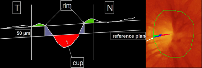
Figure9 and 10: Showing the area of the reference plane and in the cross-section.

It analyses the area marked within the contour lines (which is kept constant over successive visits) and provides a set of stereometric measures, representing cup in red colour and rim in green and blue. Disc area (total area enclosed by the contour line), Cup area (red coded area), Rim area (green and blue coded area) and Cup/Disc area ratio (ratio between cup area and total disc area) are measured as shown in the figure alongside.

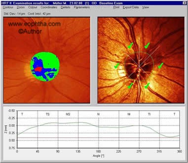
Figure11: Showing the Disc area, Cup area and Rim area which is calculated by the computer according to the color-coding.

Cup volume (volume enclosed by the contour line and located beneath the reference plane) and Rim volume (volume enclosed by the contour line and located above the reference plane) are shown in the figure. Cup shape measure is the only stereometric measure that is independent of the reference plane; a normal optic nerve head shows smaller depth values and steeper depth values are suggestive of glaucomatous disc.

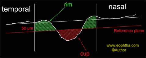
Figure12: Cup volume and Rim volume are measured with respect to the reference line.

Height variation contour (HVC- height difference between the most elevated and most depressed point of the contour line) and Mean Retinal NFL thickness (mean thickness of NFL along the contour line with respect to the reference plane) are depicted in the figure.

Multivariate analysis of the above listed stereometric measures has a sensitivity and specificity of 87% and 84% respectively in diagnosing glaucoma.3 Comparison of these parameters was carried out amongst normal, early, moderate and advanced glaucoma.4

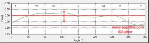
Figure13: HVC and Mean RNFL thickness calculated with respect to the reference plane.

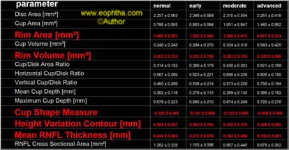
Figure14: The most important five parameters are highlighted.

Ranked sector distribution curves are another way of representing data by the HRT. Thirty sectors are plotted over the disc as shown in the adjoining figure. The data from this map is represented in line graphs,in which the red lines depict the 5th and the 95th percentiles; the blue line represents the 50th percentile and the green line being that of the tested eye. Various parameters can be depicted in this way.

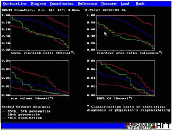
Figure 15 and 16: Showing the sectors and line diagrams of the distribution.

Based on both, the stereometric analysis and the ranked sector distribution, the computer is trained to detect and give a diagnosis of normal, glaucoma and glaucoma suspect. Discriminate analysis in HRT-1 found three parameters as being most useful to detect glaucoma:
Cup-Shape measure
Retinal surface height variation contour
Rim volume with a sensitivity of 87% and a specificity of 84%.5 Moorefield's regression analysis (MRA) in HRT-2 differentiated normal from glaucoma suspect by using linear regression between Optic disc area and Rim area with sensitivity of 96.3% and specificity of 84.3%.6
Though MRA had a higher sensitivity than the discriminant analysis, still, glaucoma detection requires a higher specificity (>95%) along with high sensitivity. Therefore HRT is not good for detection of glaucoma, but very useful for follow up.7

Optical Coherence Tomography (OCT):

It has been proven that RNFL loss occurs early in the course of glaucoma. In a study involving ten glaucoma suspects with normal visual fields, seven showed retinal ganglion cell loss.8 Another study in which 1344 patients of Ocular Hyper Tension (OHT) were followed up for 6 years with red-free photography and visual fields. The results showed that 83 out of 1344 progressed to develop visual field defects, 83% of these had RNFL loss on red-free which preceded the visual field defects and 60% of these preceded the visual field changes by 6 years.9 Therefore it has been established beyond doubt that RNFL loss precedes visual field defects. Red Free fundus evaluation, OCT and Scanning Laser Polarimetry are used to assess RNFL.

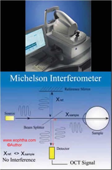
Figure17: OCT machine and the principle on which it is based.

The accuracy of OCT to detect a decrease in RNFL has been proven in literature 10-13 and that it is better than red-free fundus evaluation. The RNFL is identified by a double pass method. OCT identifies Optic nerve head margins to be where the Retinal pigment epithelium ends. It is not operator dependent. It is based on low coherence interferometry. It is analogous to the ultrasound principle, but instead of sound energy, light rays are being used. It gives a resolution of 10 microns which is much higher than that of the ultrasound (200 microns).

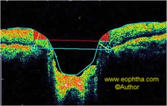
Figure18: Showing the calculation of the optic nerve head margins.

The image acquisition menu on the OCT screen gives a variety of scan options:

RNFL Thickness serial analysis (OU) Graphs of RNFL thickness are typically depicted as "double humps" in a normal scan, corresponding with the superior and inferior poles of the disc. Progressive visit line diagrams can be superimposed to get a visual impression of the decrease in the RNFL thickness.

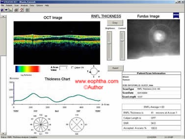
Figure19: Screen image showing the RNFL thickness in line diagram as well as sector map.

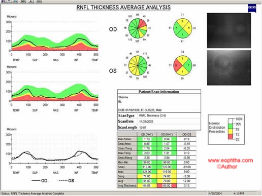
Figure20: Line diagrams of OU RNFL is depicted against the color coding. Green-normal; Yellow-borderline; Red-Abnormal

OCT proves a role in confirming the integrity of RNFL in disc suspects, provides a monitoring tool for follow up especially of patients who cannot perform reliably on visual field testing and provides a baseline for abnormal appearing discs.

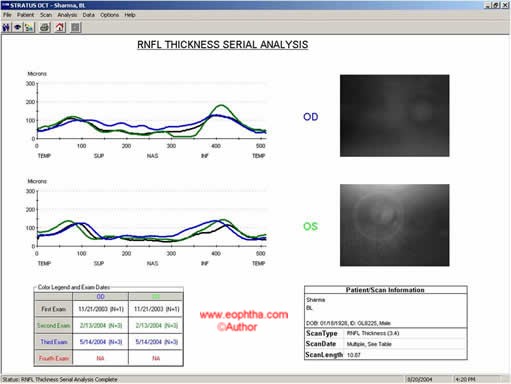
Figure21: Serial analysis showing RNFL of subsequent visits in different colors

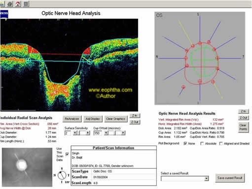
Figure22: Optic nerve head analysis

OCT and HRT correlate in the mean RNFL thickness, rim area, cup-disc ratio, and RNFL area.14,15 Though studies16 have shown a slightly higher sensitivity of OCT (sensitivity 76-79%; specificity 68-81%) as compared to HRT (sensitivity 64-75%; specificity 68-80%), by and large, it is believed that there is no significant difference.17,18

Scanning Laser Polarimetry: GDx:

The near-infrared laser light is split into two parallel rays by the optical property of birefringence of the the retinal nerve fibre layer. These two rays travel at different speeds and this difference (called retardation) directly correlates to the RNFL thickness.

Acquisition time is 0.7 seconds, after which two graphs are depicted on the screen that show the patient characteristics as compared to the normative database.

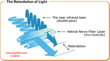
Figure23: Principle of scanning laser polarimetry

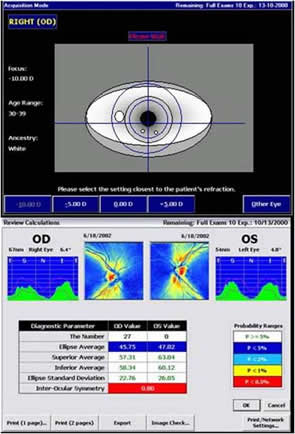
Figure24: Image acquisition screen

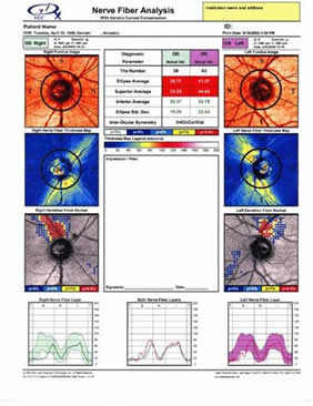
Figure24: Image acquisition screen

It gives the fundus image, colour coded thickness map of the RNFL (brighter colours represent thicker RNFL) and the comparison of the patients RNFL with that of the expected normal below. Parameters which are outside the normal range are flagged in red colour. A neural network is incorporated inside the GDx which considers hundreds of parameters and eventually assigns a number from 1 to 100. The higher the number, higher the probability of the patient having glaucoma. Serial analysis of the same patient shows the change in the RNFL over a period of time.

There is a fair topographic relationship between structural damage and functional loss. However, these diagnostic tools cannot be used in isolation to formulate a diagnosis. Both structural and functional aspects should be evaluated in order to obtain full characterisation of glaucomatous judgement for clinical diagnosis and treatment. These tools a greater role in objective follow up over a period of time.

References

1. Lisa A Kerrigan-Baumrind, Quigley HA, Mary Peace,et al.Number of Ganglion cells in Glaucoma eyes compared with threshold Visual Field tests in the same person.IOVS 2000;41:741-748.
2. Kogure S,Toda Y, Crabb D,Kashiwagi K, et al .Agreement between frequency doubling perimetry and static perimetry in eyes with high tension glaucoma and normal tension glaucoma.Br J Ophthalmology 2003;87:604-608.
3. Iester RM,Mikelberg FS,SwindaleNV,DranceSM,et al.ROC analysis of Heidelberg Retinal Tomograph optic disc shape measures in Glaucoma.Can J Ophthalmol 1997;32(6):382-388
4. Compare stereometric parameters with normal values.Richard OW Burk.Heidelberg 2000.
5. Mikelberg FS, Parfittic M, Swindale NV,et al.Ability of Heidelberg Retinal Tomograph to detect early glaucomatous Visual Field Loss.J Glaucoma 1996;4:242-247.
6. Wolstein G , Garway-Heath DF , Hitchings RA,et al.Identification of the early glaucomatous cases with the Scanning Laser Ophthalmoscope.Ophthalmology1998;105:1557-1563.
7. .Ford BA,Artes PH, Mc Cormick TA,Nicolela MT,et al.Comparison of data analysis tools for detection of glaucoma with Heidelberg Retinal Tomograph.Ophthalmology 2003;110(60)1145-1150.
8. Quigley HA,Addicks EM,Green MR,et al.Quantitative correlation of nerve fibre layer loss and visual field defects in Glaucoma,papilledema,ischemic neuropathy and toxic neuropathy.Arch Ophthalmol 1982;100(1):135-146.
9. Sommer A ,Katz A,QuigleyHA,et al.Clinically detectable NFL atrophy precedes onset of glaucomatous field loss.Arch Ophthalmol 1991 ;109:77-83.
10. Schuman JS,Pedut Kloizman T,Hertzmark E,et al.Reproducibility of nerve fibre layer using Optical Copherence Tomography.Ophthalmology1996;103:1889-1898.
11. Schuman JS,Hee MR,PuliafitoCA,et al .Quantification of nerve fibre layer thickness in normal and glaucomatous eyes using Optical Coherence Tomograph,Arch Ophthalmol 1995;113:586-596.
12. Bowd C,Weinreb RN,Williams JM,Zangwill LM,et al.The Retinal nerve fibre layer thickness in normals,ocular hypertensives and glaucomatous eyes with Optical Coherence Tomograph.Arch Ophthalmol2000;118;22-26
13. Soliman, Van Den Berg TJ,Ismail AA,De Jong LA et al.Retinal nerve fibre layer analysis:Relationship between Optical Coherence Tomography and red free photography.Am J Ophthalmology2002;133(2)187-195.
14. Mistelberger A ,Liebmann JM,Greenfield DS,Pons ME,et al.Heidelberg Retinal Tomograph and Optical Coherence Tomograph in normal ,ocularhypertensives and glaucomatous eyes.Ophthalmology1999;106(10)2027-2032
15. Schuman JS,Wollstein J,Farra T,Hertzmark E,et al.Comparison of Optic Nerve Head measurements obtained by Optical Coherence Tomograph and Confocal Scanning Laser Ophthalmoscope.Am J Ophthalmol 2003;135(4)504-51
16. Sanchez Galeana C,Bowd C,Sample PA,Weinreb RN,et al.Using Optical Imaging Summary data to detect Glaucoma.Ophthalmology2001;108(10)1812-1818
17. Schuman JS,Wollstein J,Farra T,Hertzmark E,et al.Comparison of Optic Nerve Head measurements obtained by Optical Coherence Tomograph and Confocal Scanning Laser Ophthalmoscope.Am J Ophthalmol 2003;135(4)504-512
18. Zangwill LM, Bowd C,Berry CC,Williams J,et al.Discriminating between normal and glaucomatous eyes using the Heidelberg Retinal Tomograph.GDX NerveFibre Layer analyzer.Arch Ophthalmol2001;119(7):985-993.