

Introduction:
Microsoft Excel is a vital tool for collecting and analyzing research data. It is available on the Windows platform and seamlessly works on different versions of the Windows operating system. It comes as a part of the Microsoft Office suite and is available with most basic Office versions. Though working on Excel does not require extraordinary knowledge of computers; it does require basic knowledge of the controls on the Excel workbook. Apart from that, Excel has a jargon of its own which needs to be understood to make use of all its features.
The aim of this chapter is to enable readers to understand entry, storage, and analysis of data in the Excel sheet. The chapter is divided into three sections dealing with various aspects of Excel. Readers are suggested to use this chapter for a basic overall understanding of Microsoft Excel workspace. At any point, clicking on the “Help” button in Excel will guide them to the Windows Help link on that issue.
Section 1:
Excel Components
Workbook: A workbook contains one or more worksheets.
Worksheet: The available sheet in a workbook on which data is being entered is called a worksheet.
Columns: The vertical columns of a worksheet are denoted by alphabets.
Rows: The horizontal rows of a worksheet are denoted by numbers.
Cells: Rectangular spaces in a column or row are known as cells. Cells are denoted by their position in the row and column. For example, the tenth cell in column ‘B’ will be termed as ‘B10’
Excel Workspace
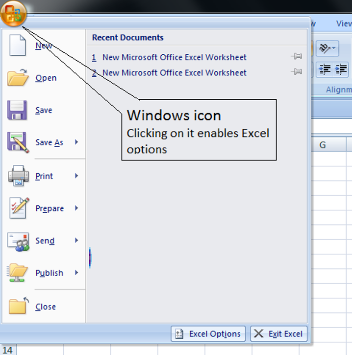
Excel options: Clicking on the icon on the top left of a workbook enables opening new or saved workbooks, saving and printing existing workbooks and other File options.
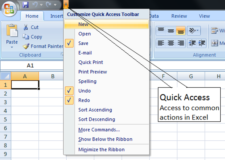
Quick Access tool bar: Frequently used workbook functions can be saved for easy access in Quick Access toolbar.
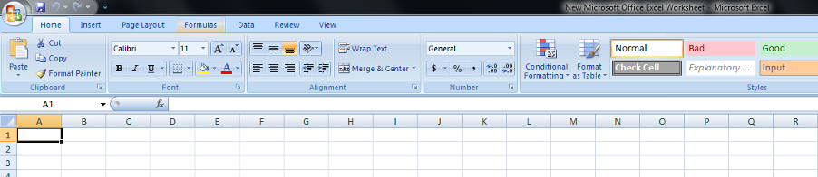
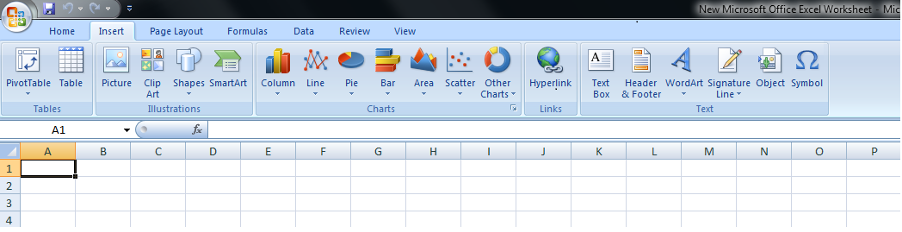
Ribbon: The Ribbon on the top contains different tabs which incorporate various commands to be used in the worksheet. The images below show Home and Insert ribbons at the top of Excel
Help: Help function is available in the extreme right of the ribbon. Clicking on Help opens a window and require an internet connection to get the reply to the queries posted in the search bar.
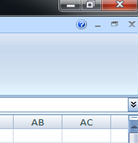
Cell editor: This space on the top allows editing individual cells.

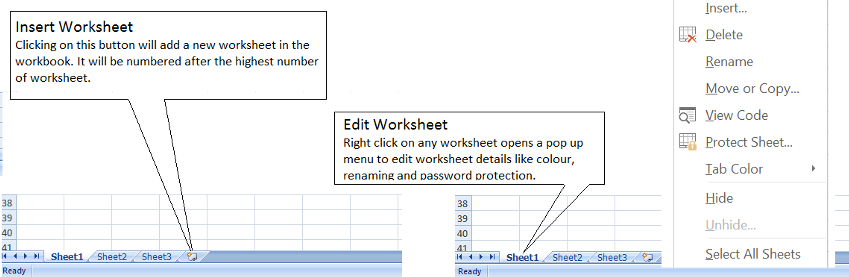
Insert worksheet: A tab on the bottom of the workbook enables the addition of new worksheets. Individual worksheets can be renamed or color-coded by double-clicking on their names in this tab.
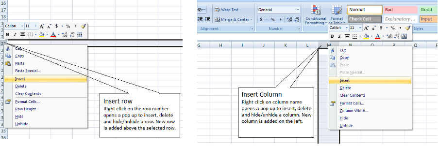
Insert new column or row: By right clicking on the name of the column a drop down menu appears. Clicking insert in this drop down menu adds a column on the left of the existing column. Similarly a row is added above the existing row.
Section 2:
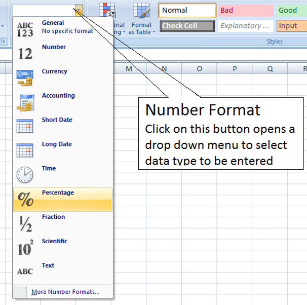
Data entryColumns are used to enter a particular assessment item whereas rows are used to enter the individual values according to each assessment item as noted in the column head. The data can be entered as various types as per the requirement so that analysis becomes easier. For example, we can highlight a specific column in the worksheet and format the Number Format in the Home ribbon to ‘percentage’ so that any number or fraction entered in that particular column will be converted to percentage after pressing Enter. The same Number Format tab can be used to enter various data types like numbers, percentage, date, time or text. The data can also be stylistically formatted for easy viewing based on the colour, font size, alignment style etc.
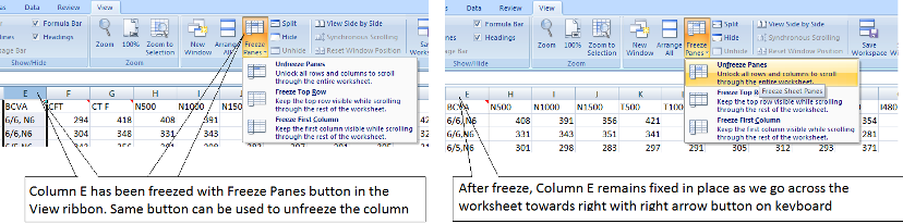
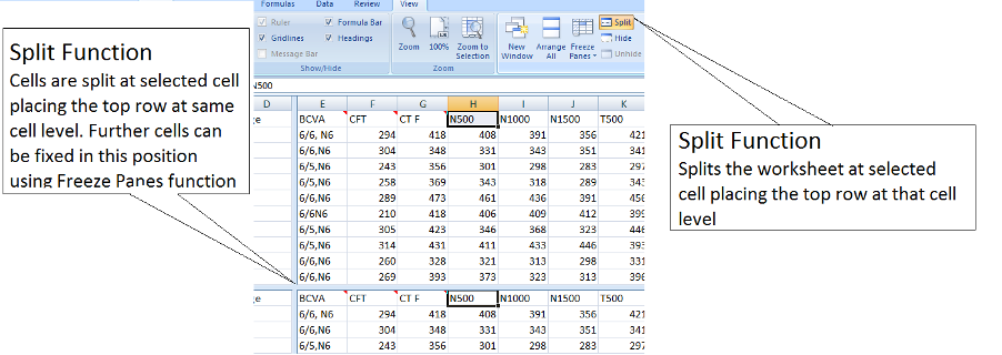
Freeze panes: This function enables us to keep the view of the column head or a specific row while we scroll down or across the worksheet. This function is available in the View ribbon on the top. We have the option of freezing the first column or top row. We can also freeze at a specific cell by first splitting the worksheet using the Split function in the View ribbon on the top. The split function also splits the worksheet and puts the top row in view at the site of the splitting of the worksheet.
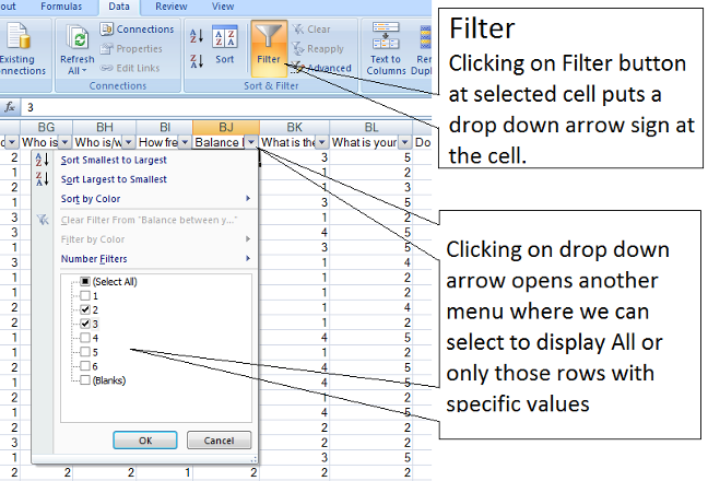
Filter data: Filtered data displays only the rows that meet the criteria that we specify and hide rows that we do not want to be displayed. After applying the filter, we can copy, find, edit, format, chart, and print the subset of filtered data without rearranging or moving it. To do this we need to go to the Data ribbon. After selecting a cell where we want to apply the filter, click on the Filter tab to apply it. After this, a drop-down arrow sign appears at the topmost cell of the column. Clicking on the arrow sign gives us the option of choosing to display either all the rows or only those rows with specific values.
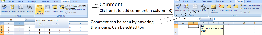
Comments: We can add comments to any cell in the worksheet. This helps in defining the values entered in a column or row to readers or to anybody other than the person entering the data.
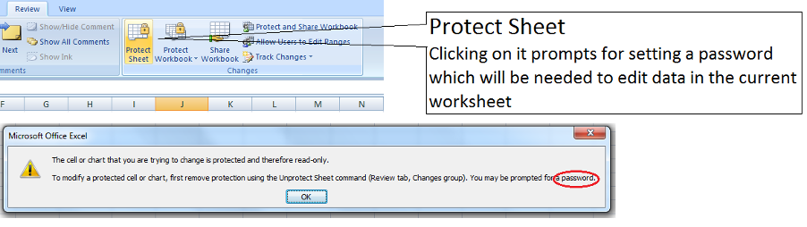
Data protection: We can prevent unauthorized modification of data in the worksheet with the help of theProtect sheet ribbon on the top. It protects the data with a password. Other users can view the data but they cannot modify without entering the valid password.
Data verification
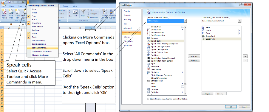
While entering the data manually in a Worksheet there is always a possibility that the entered values were incorrect. To check this sort of error, Excel has a function of speaking the data as it is entered. In addition, this Speak cell function can also be used to read back the entered data after completing the entry and the person can match the spoken values with the original data.
To enable this, click on the Quick Access toolbar. Select More commands and a customization window Excel Options will open. In the drop-down menu “Choose commands from” select All commands. Go down to the Speak commands and we can select Speak cell on Enter, Speak cells by rows or Speak cells by columns. Clicking OK will add this command to theQuick Access toolbar.
Section 3:
Constructing a formula
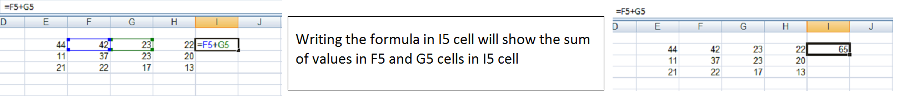
Formulae are used to analyse data entered in the cells. Each formula starts with = sign. If we want to add a formula in a cell we can click on that cell and enter the formula. For example, a formula to sum up values in cells D2 and E2 will be = D2 + E2.
Formulae follow the mathematical order which means a formula e.g. = D2+E2*A2 will first multiply the data in E2 with A2, then add the product to data in D2.
A formula can be copied and pasted in a different desired cell as per requirement. This follows relative referencing. Suppose we copy the formula = D2+E2 from cell F2 and paste it in cell F3 then resulting formula will be changed to = D3+E3.
If we want a formula to always point to same data in the same cells no matter where they are pasted then it is called absolute referencing. It is achieved by adding a dollar sign $before and after the cell. For example the formula will become = $D$2 + $E$2
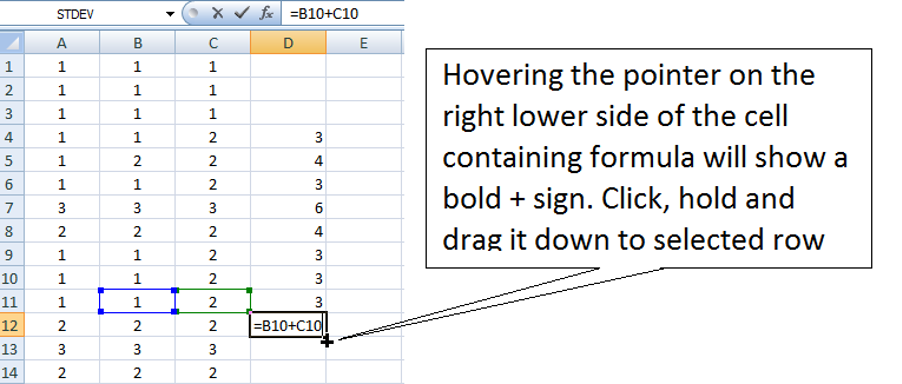
To repeat the same formula in all the cells of a column, move the pointer to the lower right side of the cell containing the formula. This will turn the pointer into a bold +. Click and hold the + and drag it up to desired row in the cell. This will apply same formula to all the cells in that column.
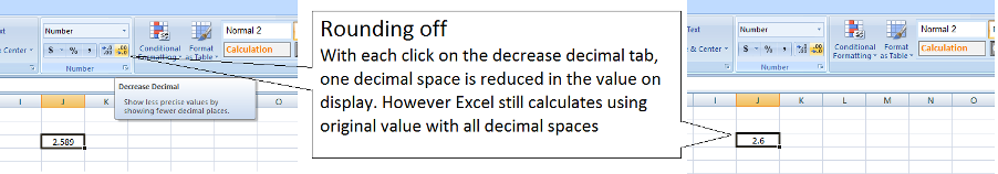
Rounding off and numeric precision of data
To reduce the decimal numbers we can click on Decrease decimal button. Each click on this button will reduce one decimal place, rounding off the data on display in the cell. However the Excel maintains a numeric precision up to 15 decimal places and while calculating it will still take in to count the decimal places irrespective of the fact that we have chosen to round off the data to fewer decimal places in the cells.
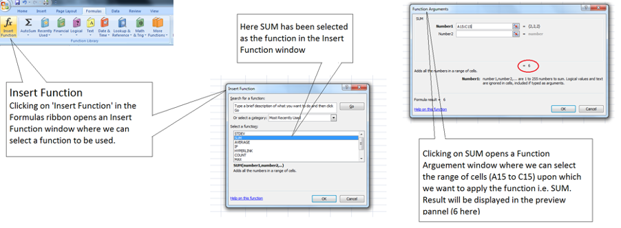
Inserting a Function
Function is a preformatted formula embedded in the Excel with an idea to minimize the complexity of lengthy formula on the worksheet. They can be entered from the Formulas ribbon on the top by clicking on Insert Function tab. Clicking on insert function opens a dialogue box on which we can Select a function. Suppose we select SUM then another Function Argument dialogue box opens. Under the Number1 type the range of cells that we want to use or we can also drag the mouse to select the range of cells to be included as the function’s arguments and click Ok. The formula result is displayed on the window as a preview.
Excel also has a variety of built-in Functions that are available in the Formulas ribbon. The built-in Functions with their description are mentioned against each function in the dialogue box which opens when we click on Insert Function for a specific function.
The pattern of typing the cell range in the Number 1 differs according to the Function selected. This pattern can be learnt from the “Help on this function” hyperlink on the bottom left of the second dialogue box used for entering the cell range. For example:
=SUM (C1, D6, G7) will add values in these three cells and give the result.
=SUM (C1:C24) will add the values from cell C1 to C24 and give the result.
=SUM (C1:C24, D1:D40) will add the sum of values in cell C1 to C24 with the sum of values in cells D1 to D40.
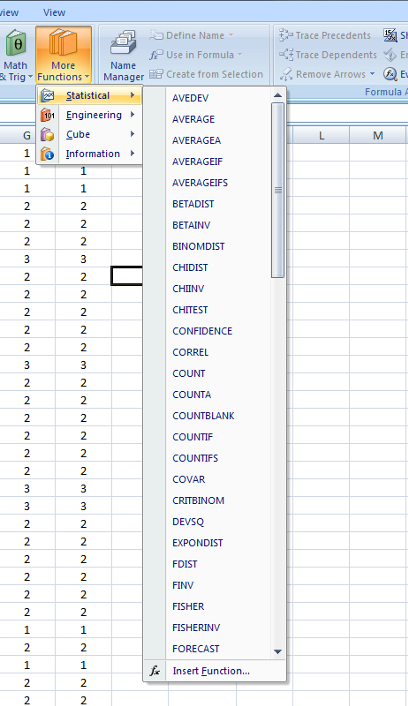
Statistical functions
Excel has a wide variety of built-in statistics functions that give, for instance, the slope and y-intercept of a line, the standard deviation of a data sample, and the mean, median and mode of a set of values. These functions are available in the Formulas ribbon under More Functions drop-down menu. Similar to the manner in which we inserted a Function in the worksheet in the previous section; we can insert a statistical function.
Excel has some built-in functions that allow a method for determining the correlation coefficient, and R-squared values of a set of data. However, the Excel workbook is not the preferred statistical analysis tool for large datasets. The reason being the fact that missing values are handled inconsistently, and sometimes incorrectly in the Excel worksheets. Moreover, most of the analyses can only be done on one column at a time. This makes it inconvenient to do the same analysis on many columns. There is no log or record of how an analysis was accomplished. It also lacks many important features for advanced analyses. However, Excel workbook is the best way of saving data and doing basic analysis. Knowledge of Excel will help in performing basic analysis and also help in understanding the functioning of higher statistical analysis software.